Episode 13: Important Notes on Linear Regression

Monday, 05/13/2024

Linear regression is about modeling the linear approximation of the causal relationship between two or more variables.

Example:

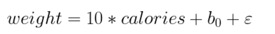
Here weight is the dependent variable and # of calories is the independent variable.

Source: Memes by Jonah Garnick ‘23

The model means that for each additional increase in calories, weight will increase by 10kg. b₀ can be thought of as the baseline weight. Keeping calorie intake aside, this would be the baseline weight of the person on average.
(ε): Error term. The expected value of errors should be zero.

• What is the difference between correlation and regression?
  • Definition:
    • Correlation measures the movement of two variables i.e. if variable1 increases , does variable2 decrease or increase with it?
    • Regression models causation i.e. change in variable1 (independent variable or regressor) causes change in variable2 (dependent variable).
  • Symmetry:
    • Correlation is symmetrical i.e. correlation of x and y is the same as correlation of y and x.
    • Regression is one way i.e. If change in x causes a change in y then the other way around may not be true.
  • Graphical Representation:
    • Correlation is calculated as a single point.
    • Regression is the best fitting line.
      
      
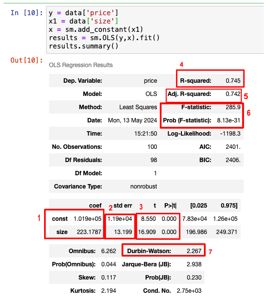
• How to interpret linear regression summary table we get from statsmodel library?

1. Coefficients: Here, ‘Price’ represents the predicted variable, and ‘Size’ is the independent variable. The table shows that the regression model will look like this:
   Price = 101900 + 223*Size

2. Standard Error: Accuracy of the prediction for each variable. The lower the error, the better the estimation.
   
3. T-statistic and p-value:
   1. We can use this to assess the significance of variables.
   2. Null hypothesis is that the coefficient is 0.
      1. When b₀ = 0, it means the regression line passes through 0. We normally don’t check this statistic for the intercept.
      2. If b₁ = 0 it would mean that size is not important in determining the price.
   3. If p-value is low i.e. 0.000 - it means we can reject the null hypothesis that the coefficient is zero and accept the alternate hypothesis i.e. choose the variable as it is significant.
      
4. R-squared: The ratio of SSR to SST (defined in the sections below). Measures the goodness of fit. Used in univariate regression.
   1. How much total variability in the dataset have we captured through the model?
   2. 0 = regression line explains none of variability of the data.
   3. 1 = regression line explains all of the variability of the data.
   4. More significant variables means higher R-squared and better model.
5. Adjusted R-squared: Same as R-squared but adjusted, so it can be used in multiple regression (more than 1 variable used to model the dependent variable).
   1. With each additional variable, the explanatory power of the model may increase or stay the same.
   2. Adjusted R-squared is always less than R-squared because it penalizes the excessive use of variables.
      
6. F-statistic: Test for overall significance of the model.
   1. Null hypothesis is that all coefficients are simultaneously zero. Our model has no merit.
   2. Alternate hypothesis is that at least one coefficient differs from zero.
   3. If p-value is less than 0.05, the model is significant but when comparing two models, we can compare their F-statistic and decide which model has higher F-statistic and hence is more significant.
7. Durbin-Watson test: Helps us check for auto-correlation.
   
   1. A value of 2 indicates no autocorrelation.
   2. Value < 1 or value > 2 is cause for alarm.

• How do we use the ANOVA framework to determine the quality of regression?
  We look at the following error measures:

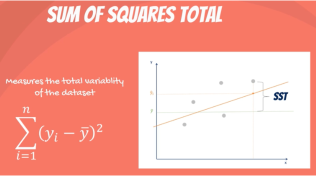
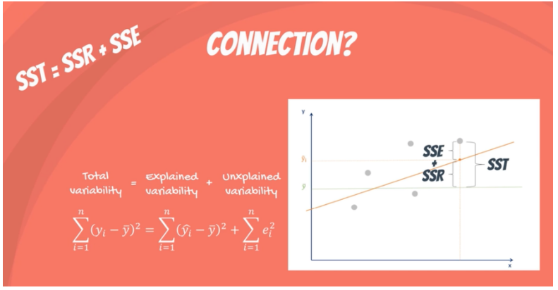
1. Sum of squares total (SST) (difference between actual value and sample mean of y).

Source: 365 Data Science

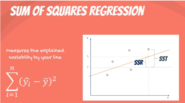
1. Sum of squares regression (SSR) (difference between predicted value and sample mean of y).

Source: 365 Data Science

1. Sum of squares error (difference between predicted value and actual value)

Source: 365 Data Science

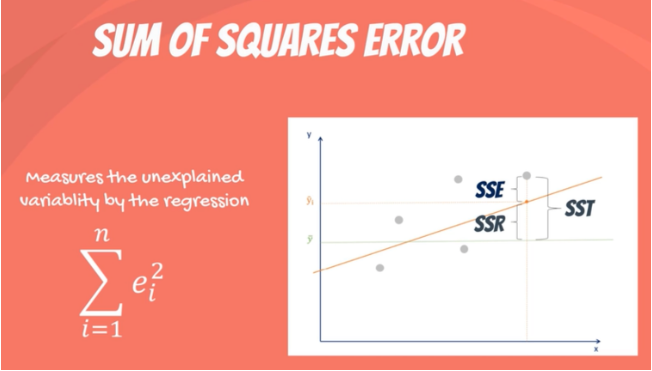
Here is how these error terms are related:

Source: 365 Data Science

In Ordinary Least Squares Regression (OLS) we minimize the sum of squared errors to reduce unexplained variability. The model chooses the line that is closest to all the points.

• What are regression assumptions?

1. Linearity:
   1. Definition: There is a linear relationship between dependent and independent variables.
   2. How to check it: Get pair plots of each independent variable with the dependent variable.
   3. How to fix: If the plots show there is a non-linear relationship, we take a log transform of the independent variable to make the relationship linear or use a non-linear regression model.
2. No Endogeneity:
   1. Definition: Collinearity of independent variable (x) and error (e) is 0 for any x or e.
   2. Omitted variable bias: Happens when we forget to include an important variable.
   3. The regressors that are used in the model are correlated with the regressor that we didn’t use in the model (omitted variable) and that is why the used regressors end up being correlated to the errors.
   4. How to check it: calculate the covariance of error and independent variables.
   5. How to fix: Include all variables in the first iteration of the model fit and then exclude some of them based on their significance.
3. Normality and homoscedasticity:
   1. Normality: Expected value of error is 0 and errors are normally distributed.
   2. Homoscedasticity: Errors should have constant variance.
   3. The conditions of normality is not required for the regression to be valid but it is required for the t-statistic etc. to be valid. If we have a large sample size then the central limit theorem applies and we can assume that errors are normally distributed.
   4. Below is an example of violation of homoscedasticity. Fixes: check OVB, remove outliers, log transformation of independent variables.

1. No auto-correlation (serial correlation):
   1. Covariance of any two error terms should be zero.
   2. Highly unlikely in cross-sectional data (data taken at one moment in time).
   3. Highly likely in time-series data.
   4. How to check: Plot residuals and look for patterns.
   5. Durbin-Watson test.
   6. How to fix: There is no fix. This condition cannot be relaxed. It’s best to use ARIMA model for time series data instead of linear regression.
2. No multicollinearity:
   1. No two variables should have a high correlation.
   2. Coefficients will be wrongly estimated if this assumption is violated.
   3. How to check: Check correlation of all pairs of independent variables.
   4. How to fix: drop one of them, transform both into one variable.

• What is a log-log model?
  In order to make the relationship between dependent and independent variable linear, we can take log of both. This is a log-log model. This can help us fulfill assumption#1 (linearity) and assumption#3 (homoscedasticity) for OLS.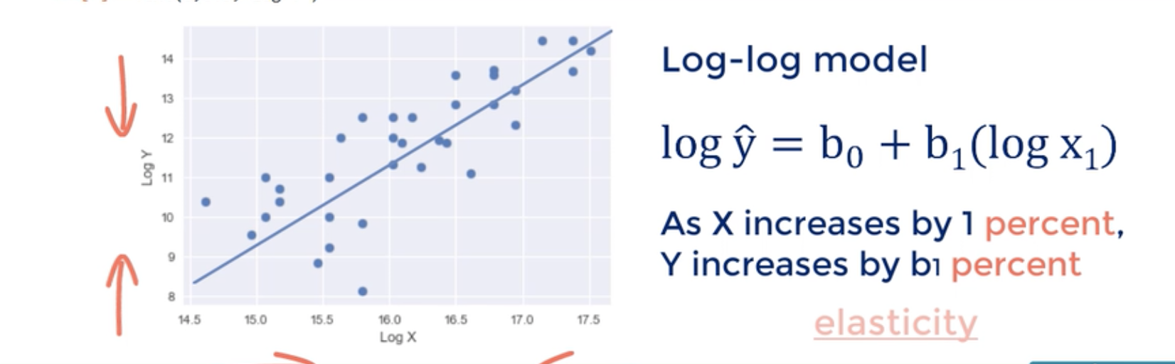

  

• What are some other techniques apart from OLS in regression analysis?

1. Generalized Least Squares
2. Maximum Likelihood Estimation
3. Bayesian Regression
4. Kernel Regression
5. Gaussian Process Regression

References:

[1] How To Perform A Linear Regression In Python (With Examples!)
[2] Data Science Career Track, 365 Data Science
[3] Memes by Jonah Garnick ‘23

Share this: