Episode 10: Notes from Deep Learning Course (Part I)

Saturday, 12/12/2020

This is part of a series of posts on some of my notes from course on Deep Learning taught by Prof. Yann LeCunn at NYU in Spring 2020 [1].

From Week 1 - 3:

Concepts:

• What are 0th order methods?

  These are gradient-free methods used to minimize a cost function. We use them when the cost function is:

  • not differentiable and has sharp discontinuities so finding its gradient is not feasible.
  • Multimodal
  • Has mixed variables.
  • Not known, when we are not sure what it looks like e.g. in reinforcement learning when we are trying to train a robot to ride a bike, our reward function outputs a reward when the robot doesn’t fall and no reward when it falls. We don’t know how to formulate this reward mechanism as a differentiable function, so we use gradient-free methods for optimization.

  Examples: Genetic Algorithms, Particle Swarm Optimization etc.

  As opposed to these methods, we have gradient-based methods such as gradient descent which can be used to optimize functions which have a known closed form, are continuous and differentiable almost everywhere. More fun stuff on it here [2].

  • What is a hyper-network?
    In a hyper-network, weights of one network G are computed as the output of another network H. H has its own set of elementary parameters and takes a copy of the inputs given to the main network G.

  

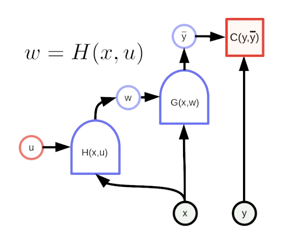
  Source: Week 3, Deep Learning Course by Yann LeCun

• What is Kaiming trick of weight initialization?

  Initializing weights is the one of the key factors that ensure that the neural network (NN) gives optimal results and converges smoothly. If we choose very large initial weights, it can lead to gradient explosion and if too small weights are chosen at the start, it can cause vanishing gradient problem.

  Kaiming trick states that when initializing an NN, we can draw these weights randomly from a normal distribution and scale them by a factor of

  So if a layer has 10 number of input nodes going into it, we can scale its initial weights (drawn from a normal distribution) by a factor of . This trick works only for layers with ReLU as an activation layer.

  LeCun’ comments:

  (“We want the variance of the output to be roughly the same as that of inputs. If the inputs to a unit are independent, the variance of the output…will be equal to the sum of the variances of the input weighted by the square of the weights. So if you have n inputs and you want the variance of the output to have the same variance, the weights should be proportional to the inverse square root of the number of inputs.”)

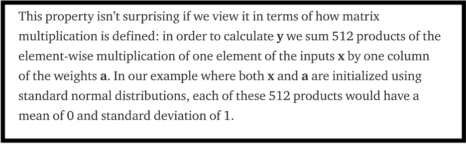
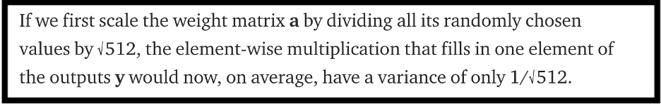
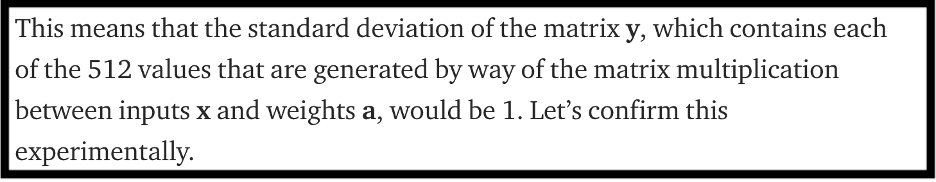
  Another easy-to-understand explanation by James Dellinger, describing the multiplication of a 521x521 weight matrix with 521x1 input vector, is as follows: [3]

  

  

Source: James Dellinger, Weight Initialization in Neural Networks: A Journey From the Basics to Kaiming

• Why do we add non-linear activations in neural nets?
  A linear layer is simply a linear combination of a set of weighted inputs. If we only have linear layers, all these layers can be squished into a single layer because combination of linear layers gives another linear layer (linear combination properties). There is no new information being added to the system if we only have multiple linear layers in the network.

• What kind of transformation is matrix multiplication? Is translation a linear transformation
  Matrix multiplication is a linear transformation. All the following transformations can be performed by simple matrix multiplication:
  • Rotation (orthonormal matrix)
  • Reflection (negative determinant)
  • Scaling/Stretching
  • Shearing

  Translation is not a linear transformation as it cannot be expressed as a product of a matrix and a vector because it involves adding scalars and 0 is not mapped to 0 after this translation. ​

• What is chain rule?
  If we have two functions C and G and we want to take their derivative w.r.t some variable w, then chain rule says that the derivative of C(G(w)) is equal to derivative of function C at point G(w), multiplied by derivative of G with respect to w. Neat, innit!

• What happens when we take the derivative of a scalar S with respect to a vector V? What is a Jacobian matrix?
  When we take derivative of a scalar (e.g. cost function) with respect to (w.r.t.) a vector (e.g. input/state vector), we get a new vector of gradients the same size as vector V.
  If we take the derivative of a vector V₁ with dimension px1, w.r.t a vector V₂ with dimension qx1, we get a matrix of size pxq (Jacobian matrix)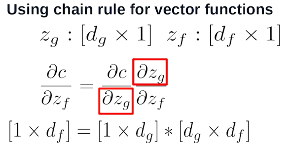

  

  Source: Here c is a scalar cost function and z_g and z_f are vectors [1].

Thought of the Week:

Generative Pre-trained Transformer 3 (GPT-3) is here! It is now the largest language model that we know of, developed by an independent lab called OpenAI in San Francisco. It has 175 billion parameters and has been trained on millions of text documents including Google books and Wikipedia articles. The underlying principle behind GPT modeling is semi-supervised learning which means to train the model on a large-sized unlabeled data in unsupervised manner and then fine-tune it by supervised learning on small set of labeled examples. [4]

Even though GPT-3 was developed for sentence completion tasks by its developers but it turns out that it can also be used to write code! Seems like it’s time for us computer scientists to get insecure about our jobs. Check out this interesting article in New York Times to know more fun stuff about GPT-3.

Until next time!

References:

[1] Yann LeCun Course
[2] 0th order methods
[3] Kaiming Trick of weight initialization
[4] GPT-3

Share this: